by Dr. Min Zhang, the EMC Consultant
Filters are almost always a part of an electronics design. Design engineers design a filter to achieve certain attenuation in a specified frequency range. We have seen that with inductive components, the impedance increases with frequency while the capacitors’ impedance decreases with frequency. By combining inductors and capacitors, we can build many types of filters, such as high-pass, low-pass or band-pass. Popular filter configurations include L-C, C-L-C (π) or L-C-L (T).
The performance of a filter is measured in terms of attenuation, or insertion loss, both of which use the units of decibels (dB). The best place to start this discussion is CISPR 17, which defines the technical terms of a filter. It also presents a detailed explanation of how to measure the insertion loss of a filter.
A filter often provides attenuation to noise in both differential mode and common mode. At a low frequency range (often between a few kHz and 1 MHz), noise is predominantly a differential mode mechanism. When the frequency goes up, common mode noise becomes more dominant.
Take a 50Ω/50Ω (source impedance/load impedance) system for instance, CISPR 17 defines two tests to measure the filter performance, which are symmetrical (differential mode) and asymmetrical (common mode). The test set-ups are shown in Figure 1. The signal generator (G) performs a signal sweep between the defined frequency range. The voltage across the load (Z2) is measured during the sweep.
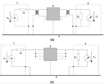
Note that in both cases Z0 and Z2 are 50 Ω. In reality, a 50Ω/50Ω system rarely exists. Therefore, the worst-case test set-ups, such as 0.1Ω/100Ω and 100Ω/0.1Ω give better filter performance analysis.
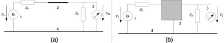
The insertion loss is defined as
| Insertion Loss = 20log(V20/v2) |
Where V20 is the voltage across Z2 before the filter is inserted, and V2 is the voltage measurement after the filter is inserted, as per Figure 2.
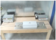
While it sounds easy and straight forward, engineers often need to see the test set-up to understand the concept better. Figure 3 shows the test set-up of an REO filter according to CISPR 17. The circuit diagram of the filter being tested is shown in Figure 4(a) and the insertion loss curve is shown in Figure 4(b).
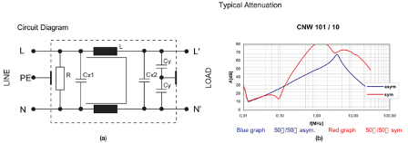
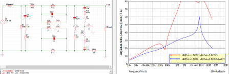
A simulated filter model is built in the SPICE simulation tool and the circuit can be found in Figure 5. As shown, when introducing parasitics into the simulation model, a close to real measurement result can be achieved. To build a useful simulation model, especially before the filter is implemented, engineers need to understand the parasitics of each passive component in the filter. If the passive components are arranged so that coupling occurs, engineers should also be aware that the filter performance could be compromised by coupling. If an off-the-shelf filter is purchased, it is a good idea to always ask the filter manufacturer for a measured attenuation curve such as the one shown in Figure 4.
Training
If you want to learn more about EMC and become an expert in troubleshooting EMI problems. Why not attend our video training course? Priced from $199, you can get 10 hour lessons. Check https://mach1design-shop.fedevel.education/itemDetail.html?itemtype=course&dbid=1644339825702&instrid=us-east-2_4pKkzzNo1:fe56227a-47c8-4ea8-ba6f-2930d01d7db8