Separate Common-mode and Differential-mode Signals

By Dr. Min Zhang, the EMC Consultant

Mach One Design Ltd

PDF download link

There are two common ways of separating common-mode and differential-mode noise. One is the voltage method; the other is the current method. 

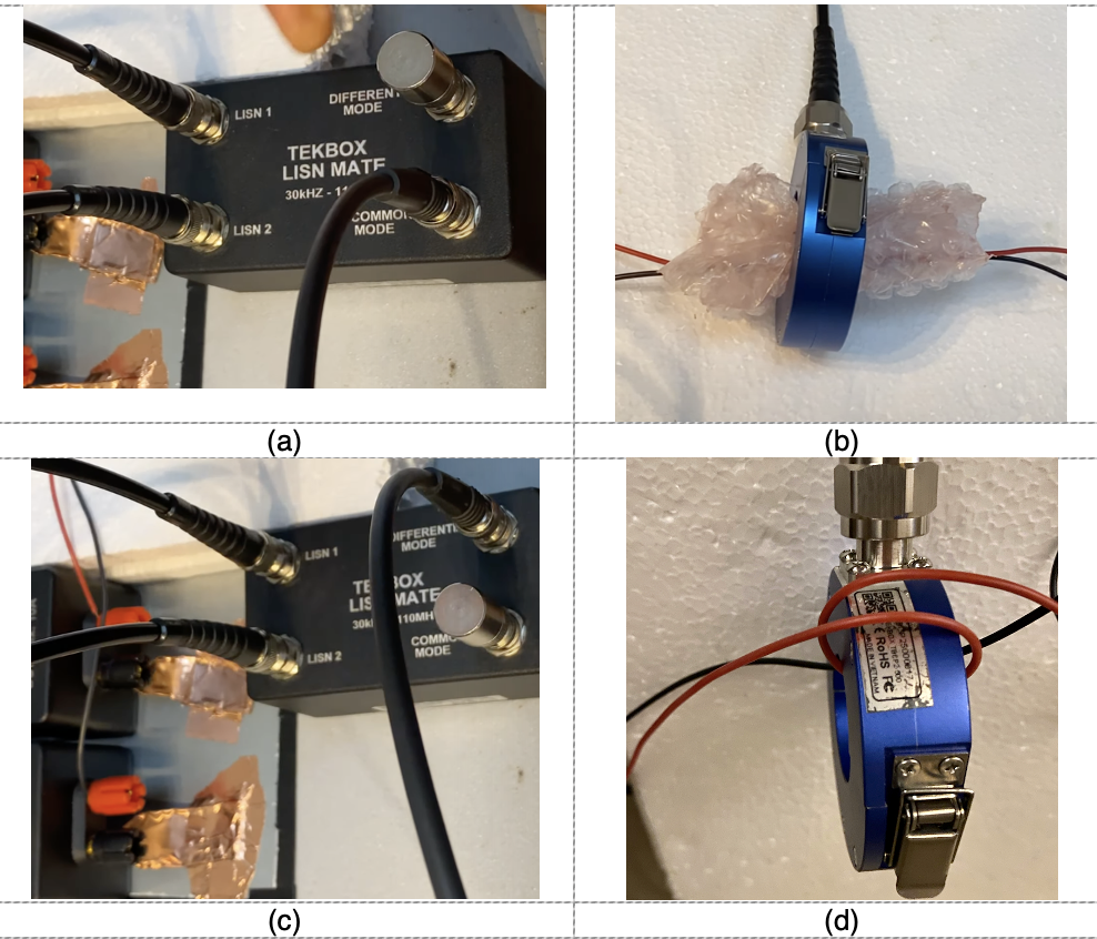
When using voltage method, a LISN-Mate is often used [1] [2] [3]. When using current method, an RF current probe can be configured to measure either common-mode or differential-mode noise depending on the wiring configuration. 

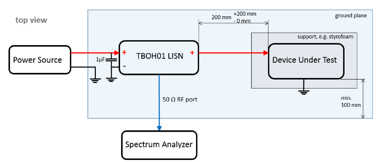
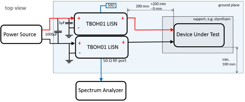
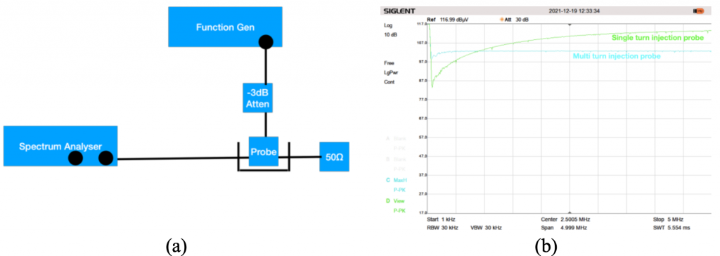
I have demonstrated how to set up the test using both methods, see https://youtu.be/0uCXs602_6M. The set-up can be found in Figure 1. This article is a follow-up, which discusses the test results and tries to make sense of it. 

Figure 1  Test set-up; (a) LISN-MATE common-mode measurement (b) current probe common-mode measurement (c) LISN-MATE differential-mode measurement (d) current probe differential-mode measurement (insulation form removed to show the configuration)

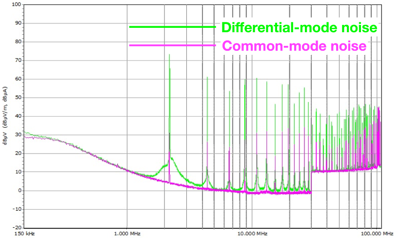
We used a buck converter as the DUT and set up the test. The LISN-MATE test result can be found in Figure2. 

Figure 2 LISN-MATE results

We then used the current probe method and compared the results with the LISN-mate result. Because current probe measures the current, we need to find a way of converting the results into voltage. This is done in the control software EMCView, where two settings are very important. 

Figure 3 The Tekbox EMCview can be set up to convert current reading to voltage

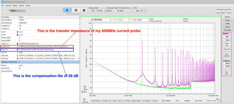
The first setting is the Lisn/Att Cor where I selected the transfer impedance file of the current probe I used. The current probe manufacturers should always provide you with the transfer impedance file of the probe you purchase. This file converts the voltage reading of a spectrum analyser to current reading (dBμV to dBμA, as dBμA=dBμV-dBΩ, where dBΩ is the transfer impedance). 

The second setting is that I added a 28 dB attenuation compensation. And the reason is:

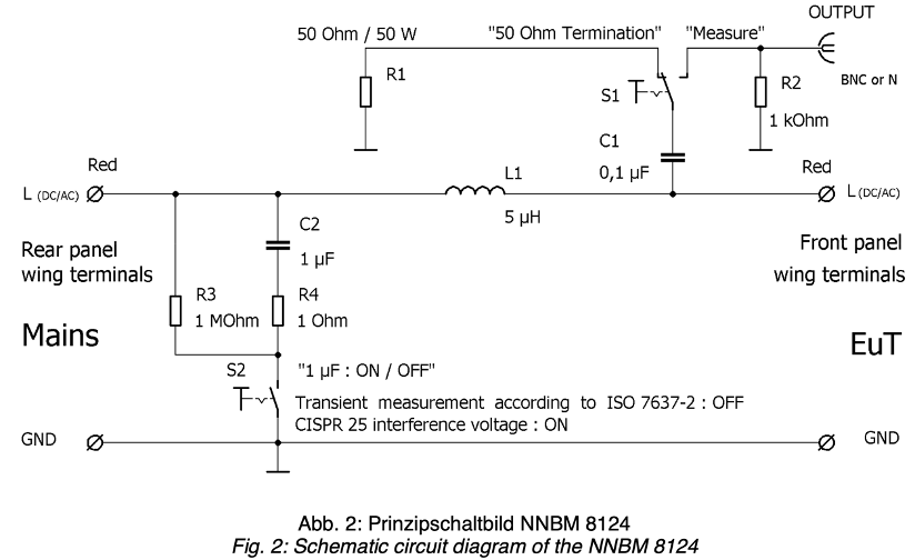
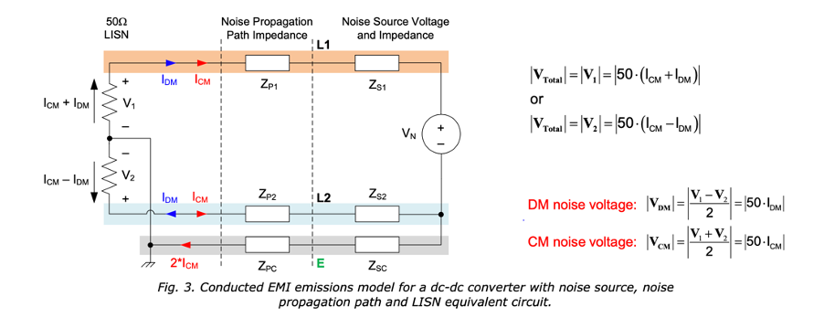
Both LISNs used for the current probe set-up are terminated with 50Ω resistors. This is important. When I measured IDM using a current probe, I have measured 2×IDM due to the wiring configuration of the current probe on the cable, so I would need to divide the value by 2, or subtract 6dB on the output. The differential voltage is measured on a 50Ω in the LISN voltage set-up, this means I will then need to add 34dBΩ (50Ω) to give me the DM voltage. That means 28dB compensation file in EMC view. 

When I measured ICM using a current probe, I also measured 2×ICM according to the picture below, so I also need to subtract 6dB on the output, then add 34dBΩ (50Ω) to give me the CM voltage reading. That means, again, 28dB compensation file in the EMC view.

Figure 4 The DM and CM voltage relationship to current [4]

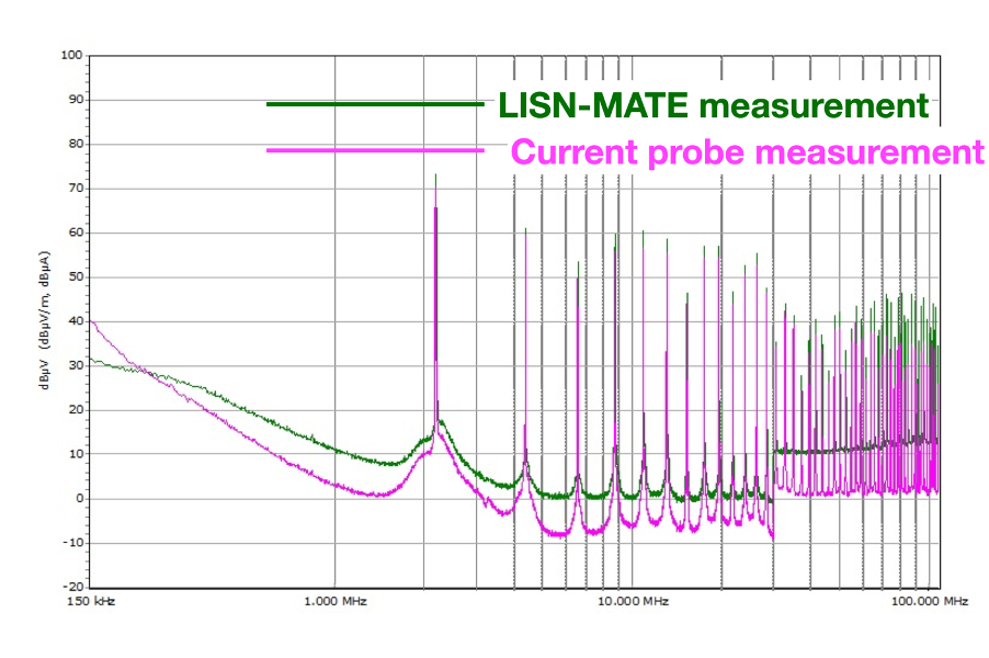
The comparison between voltage (LISN-MATE) and current measurement are shown in Figure 5 and Figure 6. Note that in order to see the difference more clearly, we turned off the attenuator in the current probe measurement, this results in a lower noise floor. 

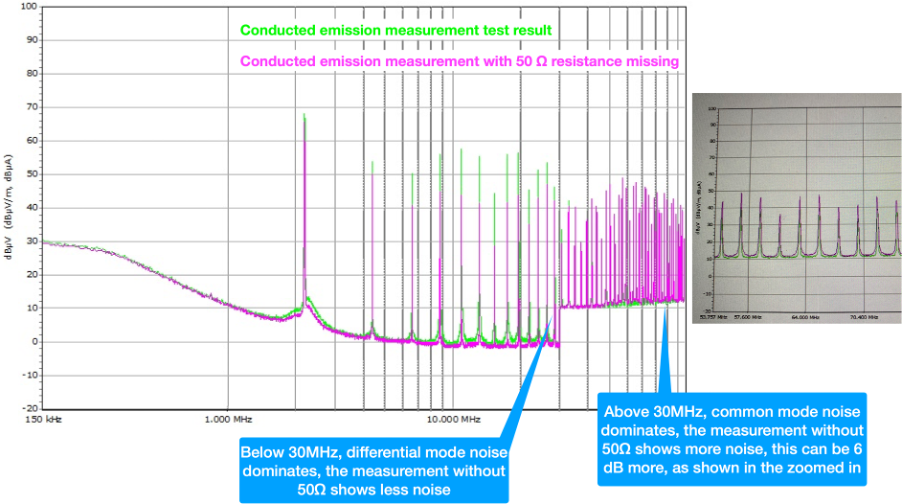
On the differential-mode noise (Figure 5), from 150kHz to 30MHz both methods are amazingly close (error difference is within 2-3 dB), from 40-100 MHz, the LISN-MATE gives 4-6dB higher reading. But from 30MHz upwards, common-mode noise starts to dominate, there will be CM to DM conversion in the system set-up, so I expected measurement difference between the two in this frequency range.

On the common-mode noise (Figure 6), it is the low frequency range (150kHz to 30MHz) that shows 6-10dB measurement difference. From 30MHz onwards, the noise is predominantly common-mode, therefore the measurement difference in this frequency range is not big. 

Figure 5 Differential-mode noise
Figure 6 Common-mode noise

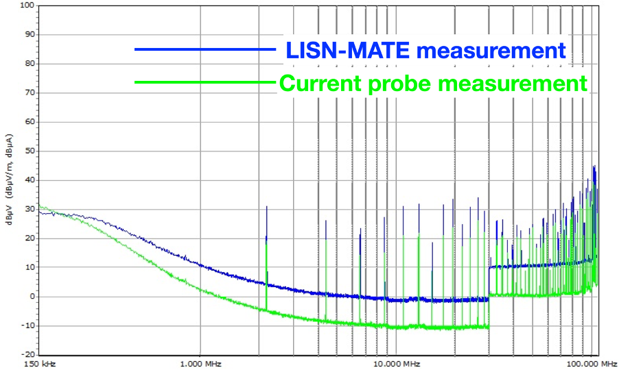
In summary, both the LISN-MATE and current probe methods can separate differential and common-mode noise well. The differential-mode noise is dominant in the lower frequency range (sub 30MHz), so I tend to trust the differential mode noise results in this region. From 30MHz, noise is predominantly common-mode, so in this frequency range, I tend to trust the common-mode noise results.  

Reference

[1] H. W. Ott, Electromagnetic Compatibility Engineering, New Jersey: Wiley, 2009. 
[2] Tekbox, “LISN-MATE,” [Online]. Available: https://www.tekbox.com/product/TBLM1_LISN_Mate_Manual.pdf.
[3] K. Wyatt, “Review: Tekbox LISN Mate is valuable for evaluating filter circuits,” [Online]. Available: https://www.edn.com/review-tekbox-lisn-mate-is-valuable-for-evaluating-filter-circuits/.
[4] T. Hegarty, “An Engineer’s Guide to Low EMI in DC/DC Regulators,” [Online]. Available: https://www.ti.com/lit/eb/slyy208/slyy208.pdf?ts=1629121242544&ref_url=https%3A%2F%2Fwww.ti.com%2Fproduct%2FLM5155.

Some details regarding to conducted emission test set-up

By Dr. Min Zhang, the EMC Consultant

Mach One Design Ltd

PDF download

I wrote in the past about how to set up conducted emission pre-compliance EMC test and made videos demonstrations https://youtu.be/KHxbk4eToXs . There are some details regarding to the test set-up. Here I summarised it below:

  1. 50Ω terminations. If two LISNs are used(as what a typical automotive application would be), make sure that one of the unmeasured LISNs (if you are measuring the 12V line, then it is the 0V line LISN) is terminated with a 50Ω resistor. Failing to do so will result in big test error. See below:
Figure 1  Error results caused by the 50 Ω termination resistor missing from the LISN

2. How important is the 1μF input capacitor to the LISN?

In some of the commercially built LISNs, there’s a switch for switching the 1μF input capacitor, shown in Figure 2. The 1μF input capacitor is used in the conducted emission test, but you have to switch it off if you are doing any kind of transient test, because the capacitor could potentially short the transient.

The Texbox LISNs I use don’t have the 1μF input capacitor built in, so it is recommended that the users should fit it themselves, as shown in Figure 3 & Figure 4 [1].

Figure 2 Schematic circuit diagram of NNBM 8124
Figure 3 Schematic of Tekbox TBOH01 and its recommended external capacitor [1]
Figure 4 Schematic of Tekbox TBOH01 and its recommended external capacitor [1]

So how important is this 1μF input capacitor for the conducted emission measurement? We consulted Tekbox and here’s what they replied:


Looking at the impedance specification of a 5μH LISN – actually I pasted the DO160 spec, because it gives a clearer picture, as it is specified down to 10kHz:

Figure 5 LISN impedance characterisitics 

From approximately 3 MHz to 110 MHz, the 5μH inductor has a high impedance and the impedance of the LISN is dominated by the 50 Ohm load impedance at the RF terminal and the capacitor is not relevant. Below 3 MHz, the impedance of the 5μH inductor decreases and in combination with the low impedance of the capacitor, the overall impedance decreases. At approximately 20kHz, the inductor impedance becomes close to zero and the capacitor starts to dominate, as its impedance increases with decreasing frequency.

I made impedance measurements with the 1μF capacitor removed. At approximately 1MHz, the impedance crosses the red limit line and you would start measuring higher spurious levels, compared to what you would measure with the 1μF capacitor.

Consequently, with or without capacitor, above 1 MHz there is no effect on the measurement result. Below 1 MHz, the measured spurious levels will be higher, compared to the correct set up. However, it will never be a lot, as there are always capacitors in the power supply – at 150 kHz it may be approximately 2~3 dB higher, if you have 1-to-2-meter supply cable length.

Interestingly, a customer came up with a similar question, as our wiring diagram seems weird at the first look:

Figure 5 LISN set up for conducted emission [1]

Above 150 kHz, the impedance of the capacitor is pretty low. Consequently, I simply replaced it by a short connection. For the LISN impedance from 150kHz to 110MHz is does not make a difference, whether you have a capacitor or a short at the source side of the LISN. For DO160 a short would be ok as well, as there is no minimum limit for the impedance below 100 kHz. However, the 1μF capacitor needs to be replaced by a 10μF capacitor, in order to avoid crossing the upper impedance limit at very low frequencies.

Replacing the capacitor by a short is also not a violation of CISPR 16, as the standard requires the LISN impedance to be within Limits with both shorted or open source terminals.

In practice, the measurement results of a set up without the 1μF are most likely fine, as long as the supply wires are short. The 5μH inductor mimics a 5m cable harness, typical for the maximum cable length you would have between car battery and an electronic device in a car. In a set-up that sees a 25 cm cable length and have the output capacitors of your power supply providing the low impedance at the source side of the inductor.”

Reference

[1] M. Mayerhofer, “Conducted emission measurement using the Tekbox 5μH LISN TBOH01,” [Online]. Available: https://www.tekbox.com/product/AN_Conducted_Noise_Measurement_Tek boxLISN_TBOH01_EMCview.pdf.

Homemade Bulk Current Injection Probe, Improved

By Dr. Min Zhang, the EMC Consultant

Mach One Design Ltd

You can download the PDF version of this article in the link below

Background

I have made a current injection probe for a quick troubleshooting job in the past, see [1], I also made a Youtube video demonstrating the test set-up, which can be found in https://youtu.be/JxfNYCbv79o .

The current injection probe was made as a quick-and-dirty approach and I never got a chance of testing the performance of it nor optimizing it. However, due to a question asked by an engineer about the wire size of the probe, also a recent article published by Arnie Nielsen [2], I decided to have a closer look at the injection probe. The aim is simple, to test the performance of it and improve it if possible.

The key point made in Arnie’s article is that by having a multiple-wire configuration, the VSWR is getting large and the performance of the injection probe starts getting detrimental. I believe this is true. In fact, I contacted Arnie and he kindly shared with me the paper his probe was based on [3]. A quick check on those properly made commercial products also indicates a ratio of 1:1. So the best approach we can take is to have a direct comparison test between the single-wire and multi-wire configuration.

The build

Construction of a single-turn winding is easy, here we used a copper that is about 1.5 cm wide and 12 cm long. Be careful about the sharp edges of the copper when making the winding. The best is to use Kapton tape to wrap around the copper, this provides both protection against the sharp edge and insulation. After that, wind the copper around the core (same core as my previous build, i.e. 28A5131-0A2) and solder a BNC connector to the single turn winding, see Figure 1.

Figure 1 Build a single-wire configuration of a current injection probe

A test jig was also built based on [2], as it can be seen from Figure 2. The two current probes under test were shown in Figure 3.

Figure 2 A test jig was built to test the performance of the current probe, a 3dB attenuator was used between the power amplifier to prevent mismatch, a 30dB attenuator was used before the spectrum analyser RF input to prevent excessive high-level of signals damaging the RF front of the spectrum analyser
Figure 3 Two probes are under test, left – multi-wire configuration, right – single-wire configuration

Test set-up

We will need two RF amplifiers to test the frequency range from 100kHz up to 1 GHz. To make things easy, I was using Texbox EMCView software to automatically generate the reference signal (in which frequency, amplitude and dwell time can be set). Two spectrum analysers were used in this case, one is to serve as an RF signal generator (by using its tracking generator output). The other one is used to monitor the injected current on the test jig.

Figure 4 Left, two RF amplifiers from Tekbox covers the range from 100kHz to 1GHz; Right, the test set-up

Performance Comparison

In the frequency range between 100kHz and 10MHz, single-turn winding configuration generates about 12dB more current compared with multi-turn configuration, but at the beginning of the spectrum (from 100kHz to 700kHz), the performance of the single-turn winding is not that good. Note that we measured the injected current in the test jig. The reading needs to be post analysed to get the true injected current level, but for a comparison study, we just look at the dB difference between the two probes.

 Figure 5 Comparison between single-turn winding and multi-turn winding injection probe, 100kHz – 10MHz

In the frequency range of 10MHz and 100MHz, single-turn injection probe performs much better, its output is flat and achieves higher level of injection current across the full spectrum, while the multi-turn injection probe’s performance starts dropping after 50MHz.

Figure 6 Comparison between single-turn winding and multi-turn winding injection probe, 10MHz – 100MHz

In the frequency range between 100MHz and 500MHz, often a frequency range that automotive companies care about the most, one can see the single-turn winding configuration performs much better (flat and maintains a high level of current level).

Figure 7 Comparison between single-turn winding and multi-turn winding injection probe, 100MHz – 500MHz

In the frequency range of 500MHz – 1GHz, the performance comparison is shown below:

Figure 8 Comparison between single-turn winding and multi-turn winding injection probe, 500MHz – 1GHz

Injected current level

So what’s the injected current level that is achieved using a single-turn winding configuration? Assuming 100dBμV reading from the test set-up, the 100dBμV was measured on the spectrum analyser (which has a 50Ω input impedance). We had a 30dB attenuator before the reading, so the true voltage reading is 130dBμV. Since it is a quasi-matched system (50Ω on the spectrum analyser and 50Ω at the other end of the line), we can just subtract 34dBΩ(50Ω) from 130dBμV to arrive at 96dBμA, a good level that you need for automotive application.

Explanations of the performance difference

A possible explanation of the performance difference between the two probes are given below.

A simplified current probe circuit is shown in Figure 9 [4]. One should note that this model is based on an RF current monitoring probe, rather than an injection probe, but the principle is the same. Because the current monitoring probe is connected with a 50Ω (as the input of a spectrum analyser), the self-inductance forms an L-C circuit with the 50Ω load. This means that the impedance of the current probe against frequency becomes flat after the corner frequency (In Figure 10).

Figure 9 (a) Simplified current probe equivalent circuit (b) Thevenin circuit
frequency response [4]
Figure 10 Current probe frequency response [4]

In [4], Smith talked about the impact of resistance on the current probe frequency response. Here, we look at the impact of self-inductance on the current probe frequency response. We simulated 2 self-inductance value while keeping the resistance value the same, Figure 11 demonstrates the impact.

Figure 11 (a) small self-inductance delays the L/R corner point (b) current probe frequency response between small and large self-inductance

Using the probe as a current monitoring probe, we set up a test to compare the performance between the two probes and the result is shown in Figure 12. Frequency span is from 10kHz to 5MHz.

Figure 12 (a) Test set-up of current monitoring probe(b) frequency response of
single and multi-turn probe

When using the probe as a bulk current injection probe, the simplified current probe circuit is then shown in Figure 13. The mutual coupling depends on the magnetizing current, which at low frequency is limited mainly by the 50Ω resistance. As frequency goes up, the self-inductance starts to limit the magnetising current. Therefore, multi- turn configuration has less mutual coupling compared with single-turn configuration as shown in the test results in Figure 14.

Figure 13 Simplified circuit for current injection probe
Figure 14 (a) Test set-up of current injection probe(b) frequency response of single and multi-turn probe

For the single turn configuration of the current injection probe, the corner point is at roughly 700kHz. This explains what is shown in Figure 5.

After 40MHz, the interwinding capacitance starts to take effect, that’s why in Figure 6, the performance of the multi-turn configuration winding starts to drop. At higher frequency, the L-C tank circuit behaviour of the multi-turn configuration means the output is oscillating.

Reference

[1]  M. Zhang, “EMC Compliance,” 2021. [Online]. Available: http://emccompliance.co.uk/a-low- cost-bulk-current-injection-test-set-up.

[2]  A. Nielsen, “InCompliance Magazine,” 12 2021. [Online]. Available: https://incompliancemag.com/article/application-of-thrifty-test-equipment-for-emc-testing/.

[3]  Frederic Lafon;Younes Benlakhouy;Francois De Daran, “ResearchGate,” [Online]. Available:https://www.researchgate.net/publication/280094695_INJECTION_PROBE_MODELING_FOR _BULK_CURRENT_INJECTION_TEST_ON_MUL TI_CONDUCTOR_TRANSMISSION_LINES .

[4]  D. Smith, “Current probes, more useful than you think”.