Techniques of using magnetic field loops
by Dr. Min Zhang, the EMC Consultant
Theory
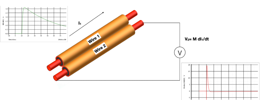
The simplest form of a transformer is a pair of wires placed in close proximity. When a changing current I1 goes through conductor 1, there is voltage induced on conductor 2 (assuming conductor 2 is open circuit). The induced voltage is defined as
V2 = M dI1/dt,
where M is the mutual inductance between the two conductors.
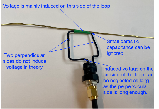
Therefore, a square magnetic field loop shown in Figure 2 is ideal to measure the induced voltage on one side of the loop, which is proportional to the rate of change of flux generated by rapidly changing current in the wire under test. Such a loop is called magnetic field loop, or “H-field loop”. But it is more accurate to be called a “dΦ/dt” loop.
It is important to emphasize here that the output of the square magnetic field loop is a voltage measurement (assuming the other end of the coaxial cable is connected to either a spectrum analyzer or an oscilloscope with a 50-ohm impedance).
Since the mutual inductance M is less than the inductance of either conductor, the output of a magnetic field loop is a lower bound for the voltage per unit length across the inductance of a current carrying conductor [1].
Note, a few assumptions are needed to make the sense of a magnetic field loop.
- The circumference of the loop is significantly less than ½ wavelength at the frequency of interest. This is because the loop could self-resonate. For instance, for a 8 cm long loop, the self-resonant frequency is about 2GHz. This means the loop can be useful up to at least 1 GHz.
- The opposite side of the loop is far enough away so the induced voltage on the far/opposite side of the loop is neglected (see Figure 2).
- The perpendicular sides of the loop do not induce voltages (see Figure 2).
- The parasitic capacitance between the magnetic field loop and the wire is ignored.
According to [1], a magnetic field loop can be modelled as shown in Figure 3. In this case, a 8 cm magnetic field loop is simulated (with circa 2 cm long conductors on each side). The 10 nH inductance value is the mutual inductance M. The 70 nH is the self-inductance of the loop. The 50 ohm impedance (of either a spectrum analyzer, or an oscilloscope with 50 ohm impedance) forms an L-C filter with the inductance of the loop. This causes the cut-off frequency shown in the frequency response.
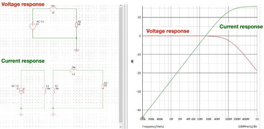
As it can be seen, the voltage response of a magnetic field loop is flat until the cut-off frequency (in this case, around 100 MHz). Above this frequency, the sensitivity of the loop starts to drop at a rate of -20dB/dec. This means the loop is useful for voltage measurement till at least 100 MHz.
The current response of the magnetic field loop (shown in green in Figure 3) means that a magnetic field loop can be used to measure (or to put it more precisely, estimate) high frequency current (whose frequency contents extend beyond the cut off frequency of the magnetic field loop). However, in general, this is not a preferred approach. This is because the mutual and self inductance of a loop is difficult to quantify (really depends on the loop construction and how one places the loop on the PCB, or next to a wire). Thus, the transfer impedance (the ratio between measured voltage to the current) of a magnetic field loop is almost impossible to calculate.