By Dr Min Zhang, the EMC Consultant
PDF download link is shown below
Background
Filters are almost always a part of electronics design. Design engineers design a filter to achieve certain attenuation in specified frequency range. There are many types of filters, such as high-pass, low-pass or band-pass. Popular filter configurations include L-C, C-L-C (π) or L-C-L (T). It is safe to say that when it comes to filter design, the discussion of the subject could easily become a very thick book.
In this article, we only want to discuss one fundamental subject, which is the performance of a filter. The performance of a filter is measured in terms of attenuation, or insertion loss, both of which use the units of dB.
Theory
The best place to start this discussion is CISPR 17, which defines the technical terms of a filter. It also presents detailed explanation of how to measure the insertion loss of a filter.
A filter often provides attenuation to noise in both differential mode and common mode. At low frequency range (often between a few kHz and 1 MHz), noise is predominantly differential mode. When the frequency goes up, common mode noise becomes more dominant.
Take a 50Ω/50Ω (source impedance/load impedance) system for instance, CISPR 17 defines two tests to measure the filter performance, which are symmetrical (differential mode) and asymmetrical (common mode). The test set-ups are shown in Figure 1. The signal generator (G) performs a signal sweep between defined frequency range and the voltage over the load (Z2) is measured.
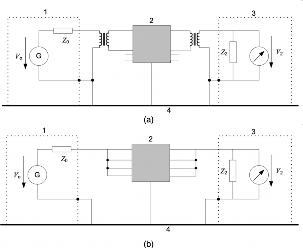
Note that in both cases Z0 and Z2 are 50 Ω. In [1], the author(s) question the 50Ω/50Ω test set-up, arguing that worst-case test set-ups, such as 0.1Ω/100Ω and 100Ω/0.1Ω give better filter performance analysis. It is a valid point, since in reality, a 50Ω/50Ω system barely exists.
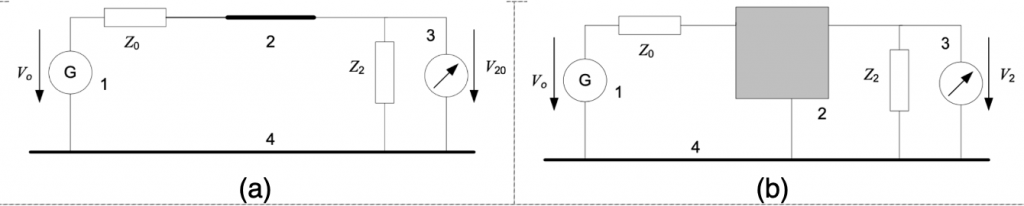
Regardless of the test set-up, the insertion loss is defined as
Insertion loss = 20log(V20/V2),
Where V20 is the voltage over Z2 before the filter is inserted, V2 is the voltage measurement after the filter is inserted. Test set-ups are shown in Figure 2.
Practical Application
While the theory sounds easy and straight forward. In order to get a feel of what insertion loss of a filter is all about, here we present a practical example to demonstrate.
The filter we demonstrate is an off-the-shelf Schaffner part FN 670-3Amp. The filter and its electric schematics are shown in Figure 3.
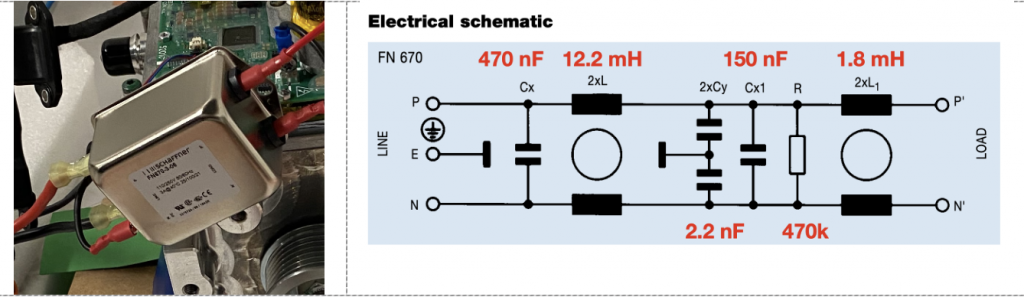
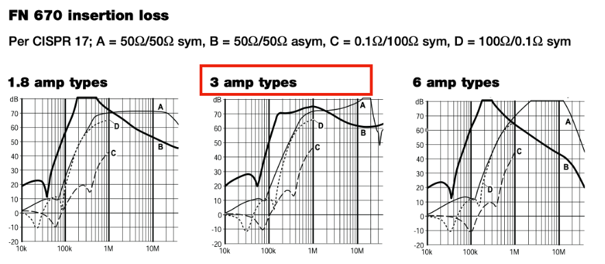
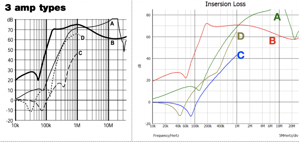
Figure 4 shows the filter performance according to the supplier datasheet. As it can be seen, four test set-up results are presented to give the best filter analysis. It should be noted that for set-up C and D, the insertion loss is only performed between 10kHz and 1 MHz. As we mentioned earlier, this is because when frequency goes beyond 1 MHz, common mode noise starts dominating, therefore the measurement results for the symmetrical mode beyond 1 MHz can over predict the filter performance.
A SPICE based simulation model is then modelled to demonstrate the insertion loss. The filter needs to be carefully built with the consideration of parasitic parameters, since above 500kHz, parasitic parameters of the passive components in the filter start taking effect. The simulation model is shown in Figure 5. For details of the simulation model and how to tune the parasitic parameters, refer to [2].
The filter insertion loss analysis can be easily performed using the SPICE based AC analysis tool. The simulation model is shown in Figure 6. Selected frequency sweep can be completed within seconds, and the insertion loss is plotted either using the simulation probe tool or simply using the equation of 20log(mag(V1/V2)).
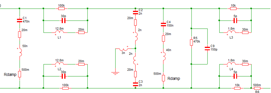
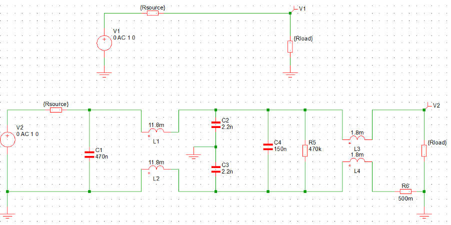
Figure 7 shows the simulated results compared with the datasheet measurement results. As it can be seen, a high level of matching is achieved.
Limitations
The technical problem of this sort of simulation is that the magnetic characteristics cannot be fully modelled. For instance, 30pF interwinding capacitance for a 12.2 mH CMC and 5 pF interwinding capacitance for 1.8 mH CMC simply cannot be true as I was expecting at least 150 pF for the 12.2 mH CMC. But only these capacitance value can make sure the resonant frequency point in the simulation matches with the test results. Therefore, the interwinding capacitance values are not reasonable. In [2], I provided possible explanation. I think it is because the leakage inductance reduces quite significantly with the frequency (backed up by some literature review), therefore, the interwinding capacitance value could be a lot bigger than the simulation model, since simulation assumes fixed inductance against frequency. This same problem also causes about 10 db over prediction of the filter performance as explained in the article.
In order to improve the simulation model, one will then need to build a frequency dependent magnetics model, which will cost time and effort if one doesn’t have an existing model, therefore, defeating the very purpose of building a quick and easy SPICE model for filter performance analysis. Saying that, it is on my list to explore this area further.
Conclusion
In this article, the basics of filter insertion loss and measurement set-ups are introduced. Simulation model is presented to demonstrate the filter performance. The simulated insertion loss of the filter matches the test results very well.
Reference
| [1] | Schaffner, “CISPR 17 Measurements 50Ω / 50Ω versus 0.1Ω / 100Ω,” [Online]. Available: https://www.schaffner.com/fileadmin/media/downloads/application_note/Schaffner_AN_CISPR17_Measurements_E8.pdf. |
| [2] | M. Zhang, “A simple and effecitve SPICE based simulation model to assist your filter design,” SignalIntegrity. |